General Social Survey

Introduction
The General Social Survey (GSS) gathers data on American society in order to monitor and explain trends in attitudes, behaviours, and attributes. Many trends have been tracked for decades, so one can see the evolution of attitudes, etc in American Society.
The General Social Survey
In the following section we will use the GSS survey data sample to predict population parameters for people’s social media usage. We will be creating 95% confidence intervals for population parameters. The variables we have are the following:
emailhrandemailmin: hours and minutes spent on email weekly. For example, if the response is 2.50 hours, this would be recorded as emailhr = 2 and emailmin = 30snapchat,instagrm,twitter: whether respondents used these social media in 2016sex: Female - Maledegree: highest education level attained
The data
In this assignment we analyze data from the 2016 GSS sample data, using it to estimate values of population parameters of interest about US adults. The GSS sample data file has 2867 observations of 935 variables, but we are only interested in very few of these variables and therefore use a smaller file.
The process
First, we load the dataframe…
gss <- read_csv(here::here("data", "smallgss2016.csv"),
                na = c("", "Don't know",
                       "No answer", "Not applicable"))
Let’s have a look at the dataframe…
glimpse(gss)## Rows: 2,867
## Columns: 7
## $ emailmin <chr> "0", "30", "NA", "10", "NA", "0", "0", "NA", "0", "NA", "0...
## $ emailhr <chr> "12", "0", "NA", "0", "NA", "2", "40", "NA", "0", "NA", "2...
## $ snapchat <chr> "NA", "No", "No", "NA", "Yes", "No", "NA", "Yes", "NA", "N...
## $ instagrm <chr> "NA", "No", "No", "NA", "Yes", "Yes", "NA", "Yes", "NA", "...
## $ twitter <chr> "NA", "No", "No", "NA", "No", "No", "NA", "No", "NA", "No"...
## $ sex <chr> "Male", "Male", "Male", "Female", "Female", "Female", "Mal...
## $ degree <chr> "Bachelor", "High school", "Bachelor", "High school", "Gra...# Glipmse the first data rows in order to check data structure
check_gss <- head(gss, 10)
check_gss %>%
# Use Kable package in order to transofrm into nice table
kbl(col.names = c("E-Mail (min)", "E-Mail (hr)", "Snapchat", "Instagram", "Twitter", "Sex", "Degree")) %>%
kable_material_dark() %>%
kable_styling(fixed_thead = T, full_width = F, font_size = 14) %>%
row_spec(0, background = "#363640", color = "white")| E-Mail (min) | E-Mail (hr) | Snapchat | Sex | Degree | ||
|---|---|---|---|---|---|---|
| 0 | 12 | NA | NA | NA | Male | Bachelor |
| 30 | 0 | No | No | No | Male | High school |
| NA | NA | No | No | No | Male | Bachelor |
| 10 | 0 | NA | NA | NA | Female | High school |
| NA | NA | Yes | Yes | No | Female | Graduate |
| 0 | 2 | No | Yes | No | Female | Junior college |
| 0 | 40 | NA | NA | NA | Male | High school |
| NA | NA | Yes | Yes | No | Female | High school |
| 0 | 0 | NA | NA | NA | Male | High school |
| NA | NA | No | No | No | Male | Junior college |
As we can observe we have data of survey respondent’s social media and email usage per week as well as basic information about the gender and educational degree. As we want intend to estimate the population proportion of Snapchat and Instagram users in 2016, we need to create a new variable (snapchat_insta) that indicates if the person is either a Snapchat or Instagram user (or both).
Estimate population proportion of Instagram and Snapchat by sex
Let’s manipulate the data …
gss_adjusted <- gss %>%
  mutate(
    # we create a new variable snap_insta that is "Yes" if the respondent reported using snapchat or instagram
    snap_insta = case_when(
    instagrm == "Yes" | snapchat == "Yes" ~ "Yes",
    instagrm == "No" & snapchat == "No" ~ "No"
    ))

# we calculate the proportion of "Yes" answers for snap_insta excluding NAs and group by gender and usage of instagram
snap_insta_proportion <- gss_adjusted %>%
  # we group by gender and snap_insta in order to calculate the individual CIs later
  group_by(sex, snap_insta) %>%
  summarise(count = n()) %>%
  filter(snap_insta == "Yes" | snap_insta == "No") %>%
  mutate(share = count/sum(count)) # %>%
  # filter(snap_insta =="Yes")

snap_insta_proportion %>%
  # Use Kable package in order to transofrm into nice table
  kbl(col.names = c("Gender", "Snap_Insta User", "Count", "Share (%)")) %>%
  kable_material_dark() %>%
  kable_styling(fixed_thead = T, full_width = F, font_size = 14) %>%
row_spec(0, background = "#363640", color = "white")| Gender | Snap_Insta User | Count | Share (%) |
|---|---|---|---|
| Female | No | 447 | 0.581 |
| Female | Yes | 322 | 0.419 |
| Male | No | 411 | 0.682 |
| Male | Yes | 192 | 0.318 |
Now that we summarized the data and grouped by Gender and whether the person is using instagram or snapchat, we calculated the distribution of users for each gender.
Let’s calculate the Confidence Intervall…
# we calculate the ci by calculating the required variables
ci_gss <- snap_insta_proportion %>%
  # filter(snap_insta == "Yes") %>%
  summarise(snap_insta,
            count,
            sum = sum(count),
            se_social = sqrt((share*(1-share)/sum(count))),
            share,
            # we calculate the t_critical for 95% CIs for men and women
            t_critical = qt(0.975, count-1),
            margin_of_error = t_critical * se_social,
            ci_lower = share - margin_of_error,
            ci_higher = share + margin_of_error
            ) %>%
  filter(snap_insta == "Yes") %>%
  select(ci_lower, share, ci_higher)

ci_gss %>%
  kbl(col.names = c("Gender", "Lower CI", "Expected share", "Upper CI")) %>%
  kable_material_dark() %>%
  kable_styling(fixed_thead = T, full_width = F, font_size = 14) %>%
row_spec(0, background = "#363640", color = "white")| Gender | Lower CI | Expected share | Upper CI |
|---|---|---|---|
| Female | 0.384 | 0.419 | 0.454 |
| Male | 0.281 | 0.318 | 0.356 |
Based on our sample set we expect ~42% or Females to use instagram/snapchat with a 95% confidence intervall betweeen (38.4%, 45.4%). For Males the expected share is ~28% with a 95% CI between (28.1%, 35.6%).
Population proprtion of Twitter users by education level
Next, we want to estimate the population proportion of Twitter users by education level in 2016.
There are 5 education levels in variable degree which, in ascending order of years of education, are:
Lt high schoolHigh SchoolJunior collegeBachelorGraduate
Let’s calculate the population proportion…
# we define the levels for the degree column by using a degree vector
level_order <- c("Lt high school", "High school", "Junior college", "Bachelor", "Graduate")

# we define a non_university vector for the bachelor_graduate classification later on
non_university <- c("Lt high school", "High school", "Junior college")

twitter_adjusted <- gss %>%
  group_by(degree) %>%
  # we turn the the degree column from a character variable into a factor variable
  mutate(
    degree = factor(degree,
                    levels = level_order)
    ) %>%
  arrange(degree) %>%
  # we create a bachelor_graduate column based on the degree
  mutate(bachelor_graduate = case_when(
    degree == "Bachelor" ~ "Yes",
    degree == "Graduate" ~ "Yes",
    degree %in% non_university ~ "No"
    )) # %>%
  # Filter to check NA values
  # filter(is.na(degree))

  # check if previous mutate function worked correctly
  #group_by(degree) %>%
  #summarize(count(bachelor_graduate == "Yes"))

#twitter_adjusted

# just an alternative possibility to filter out the NA rows for twitter/ bachelor_graduate
# yes_no <- c("Yes", "No")
#ci_twitter_2 <- twitter_adjusted %>%
#  group_by(twitter, bachelor_graduate) %>%
#  filter(twitter %in% yes_no & bachelor_graduate %in% yes_no)

# we calculate the proportion of twitter users among bachelor_graduates
twitter_bg_proportion <- twitter_adjusted %>%
  select(twitter, bachelor_graduate) %>%
  group_by(bachelor_graduate, twitter) %>%
  filter(!is.na(bachelor_graduate),
         twitter != "NA",
         bachelor_graduate == "Yes") %>%
  summarise(count = n()) %>%
  mutate(share = count/sum(count))

#twitter_bg_proportion

# we calculate the ci for bachelor_graduates regarding the usage of twitter
ci_twitter <- twitter_bg_proportion %>%
  summarise(count,
            se_twitter = sqrt((share*(1-share)/sum(count))),
            share,
            twitter,
            t_critical = qt(0.975, count-1),
            margin_of_error = t_critical * se_twitter,
            ci_lower = share - margin_of_error,
            ci_higher = share + margin_of_error
            ) %>%
  select(twitter, ci_lower, share, ci_higher)

#ci_twitter

ci_twitter %>%
  kbl(col.names = c("Bachelor-Master Grad", "Twitter User", "Lower CI", "Expected share", "Upper CI")) %>%
  kable_material_dark() %>%
  kable_styling(fixed_thead = T, full_width = F, font_size = 14) %>%
row_spec(0, background = "#363640", color = "white")| Bachelor-Master Grad | Twitter User | Lower CI | Expected share | Upper CI |
|---|---|---|---|---|
| Yes | No | 0.729 | 0.767 | 0.804 |
| Yes | Yes | 0.195 | 0.233 | 0.271 |
The 95% confidence intervals for Twitter/ Non-Twitter users among people with a bachelor or graduate degree do not overlap as the expected share of twitter users based on the sample set is ~77% and thus the CI will not overlap with the CI around the expected share of Non-Twitter users of ~23%.
Estimation of weekly email usage of Americans
In the following we estimate the population parameter on time spent on email weekly of Americans.
Let’s manipulate the data and plot the email usage…
#we change the NA strings into actual NA values
gss_adjusted[gss_adjusted == "NA"] <- NA

# we create a new dataframe to calculate the time spent on email per week for the users
gss_email <- gss_adjusted %>%
  na.omit() %>%
  mutate(emailmin = as.integer(emailmin),
         emailhr = as.integer(emailhr),
         email = emailmin + emailhr*60)

ggplot(gss_email, aes(email))+
  geom_boxplot() +
  labs(x = "Minutes (per week)", title = "Clear signs of outliers in the dataset influencing the mean e-mail usage", subtitle = "Distribution of weekly email usage of Americans") +
  theme_bw()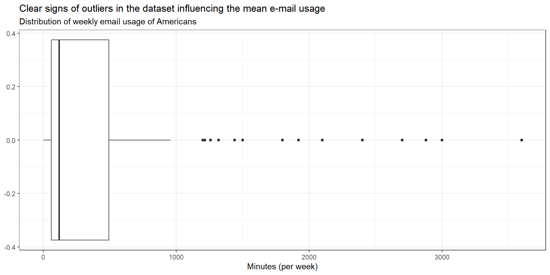
mean_median_email <- gss_email %>%
  summarise(mean = mean(email), median = median(email))

mean_median_email %>%
  kbl(col.names = c("Mean min per week", "Median min per week")) %>%
  kable_material_dark() %>%
  kable_styling(fixed_thead = T, full_width = F, font_size = 14) %>%
row_spec(0, background = "#363640", color = "white")| Mean min per week | Median min per week |
|---|---|
| 445 | 120 |
Looking at the distribution of email minutes spent per week it is better to use the median number as a measure of the typical amount of time Americans spent. As can be observed in the graph above, there are several outliers leading to the expected difference of mean (445 min) vs. median (120 min).
Let’s calculate the CI using the bootstrap method…
# calculate bootstrap confidence interval

bootstrap_email_ci <- gss_email %>%
  # specify the variable of interest, here email minutes spent per week
  specify(response = email) %>%
  generate(reps = 100, type="bootstrap") %>%
  # choose median as variable to calculate
  calculate(stat = "median") %>%
  # calculate confidence interval
  get_confidence_interval(level = 0.95, type = "percentile") %>%
  # transform from min into h + min as decimal
  mutate(lower_ci = lower_ci/60, upper_ci = upper_ci/60)

bootstrap_email_ci %>%
  kbl(col.names = c("Lower CI", "Upper CI")) %>%
  kable_material_dark() %>%
  kable_styling(fixed_thead = T, full_width = F, font_size = 14) %>%
row_spec(0, background = "#363640", color = "white")| Lower CI | Upper CI |
|---|---|
| 2 | 3 |
# Define variable to calculate hours and minutes seperately
a <- bootstrap_email_ci$lower_ci
b <- bootstrap_email_ci$upper_ci

# use mod for decimals using modulo operator
lower_ci_mod <- round(a%%1*60, digits = 0)
# use int for integer
lower_ci_int <- a%/%1

upper_ci_mod <- round(b%%1*60, digits = 0)
upper_ci_int <- b%/%1
In the goven example we calculated the 95% confidence interval. A 99% confidence interval would be expected to be wider as this would indicate that the confidence intervall in 99% of the times should include the observed median (or mean) of the respective sample.
## [1] "The median lower bound of the CI for usage of email is: 2 hours and 0 minutes"## [1] "The median upper bound of the CI for usage of email is: 3 hours and 0 minutes"Looking at the 95%-tile median confidence interval, it is interesting to note that the confidence interval is only an approximate value for the 95%-tile intervals. The reason for this lies in the fact that the median value would be given as the n/2 value of the sample. as the is no e.g. “45.5th” value of a dataset, the median confidence interval would output e.g. the nearest value, being the e.g. “46th” value of the sample. Thus, we get exact values of 2h and 3h for the CI respectively.
Last updated: 20 September, 2020