AirBnB Beijing (Part 1)

Introduction (Part 1: Data cleaning + EDA)
The following project focuses on the analysis of an AirBnB dataset. As part of the project I performed Exploratory Data Analysis (EDA), Data visualization as well as Regression Analysis. The final output is a multivariate regression model that predicts the total cost of two people to stay at an AirBnB property in Beijing for 4 nights. For the purpose of this work display I’ll present a smaller subset of analyses and visualizations that were part of the larger project.
Therefore the focus of this showcase (Part 1) is the structured data cleaning and data exploration process (EDA).
Data cleaning process
First, we load the dataframe…
beijing_data <- vroom::vroom("http://data.insideairbnb.com/china/beijing/beijing/2020-06-19/data/listings.csv.gz")%>%
  clean_names()
Let’s have a look at the dataframe…
# Skim data set to get initial understanding of dataset like missing values, datatypes etc.
# skim(beijing_data)
Looking at the initial skim of data we observe that there is a large amount of missing entries (i.e. NA values) for certain variables. Based on this initial view, we’ll remove variables that:
- Only have one distinct value/ NA or very limited number of entries (e.g. square footage)
- Binary/ Categorical variables that only have one value (e.g. “FALSE” or different Bed Types) for >95% of entries
- Descriptive (Text) strings that could only be processed with NLP (natural language processing) and which would require advanced cleaning/ time effort
- All variable with datatype date (not used for analysis), e.g. last time scraped
General observations:
- Number of rows/ observations: 36,283
- Number of columns/ variables: 106
- Column type frequency:
- Character: 46
- Date: 15
- Logical: 15
- Numeric: 40
As indicated by the count of data types, we have to further explore the variables and potentially transform them into appropriate types to prepare the dataset for further analysis (esp. character data types). We can observe that there are no factor or categorical variables on this dataset. As we will see, however, there are variables such as property type, host response time and cancellation policy for which most of the responses are represented by a limited set of options. As a first step, we’ll additionally change the datatypes from string to numeric for price, cleaning_fee, security_deposit and extra_people.
Let’s manipulate the data …
# Select potentially relevant data columns (variables) to be further analyzed in the next steps
beijing_selected <- beijing_data %>%
  #Select the relevant variables
  select(id,
         host_response_time,
         host_response_rate,
         host_acceptance_rate,
         host_is_superhost,
         host_listings_count,
         host_total_listings_count,
         host_identity_verified,
         neighbourhood,
         neighbourhood_cleansed,
         zipcode,
         latitude,
         longitude,
         is_location_exact,
         property_type,
         room_type,
         accommodates,
         bathrooms,
         bedrooms,
         beds,
         price,
         security_deposit,
         cleaning_fee,
         guests_included,
         extra_people,
         minimum_nights,
         maximum_nights,
         number_of_reviews,
         number_of_reviews_ltm,
         review_scores_rating,
         review_scores_checkin,
         review_scores_cleanliness,
         review_scores_accuracy,
         review_scores_communication,
         review_scores_location,
         review_scores_value,
         instant_bookable,
         cancellation_policy,
         reviews_per_month) %>%
  # Perform basic mutate to change data type of numeric variables and parse number
  mutate(price = parse_number(price),
         cleaning_fee = parse_number(cleaning_fee),
         security_deposit = parse_number(security_deposit),
         extra_people = parse_number(extra_people),
         host_response_rate = parse_number(host_response_rate),
         host_acceptance_rate = parse_number(host_acceptance_rate)
         )
Following this initial clean, we create a bar chart showing the % of missing values for further data cleaning.
Let’s visualize the missing values in the dataset…
# We plot a bar chart that shows the percentage, thanks to Group 9 for the inspiration

missing_entries <- beijing_selected %>%
  summarise_all(~(sum(is.na(.))/n())*100) %>%
  pivot_longer(cols = id:reviews_per_month, names_to = "variable", values_to = "perc_missing_values") %>%
  group_by(variable)


missing_entries %>%
           ggplot(aes(x = reorder(variable, perc_missing_values), y = perc_missing_values, show.legend = FALSE)) +
           geom_bar(stat = "identity") +
           coord_flip() +
           labs(title = "Numerous selected variables in AirBnB dataset have >40% missing values", subtitle = "Percentage of missing values (NAs) is AirBnB dataset", y = "Percentage (%)", x = element_blank()) +
           theme_bw()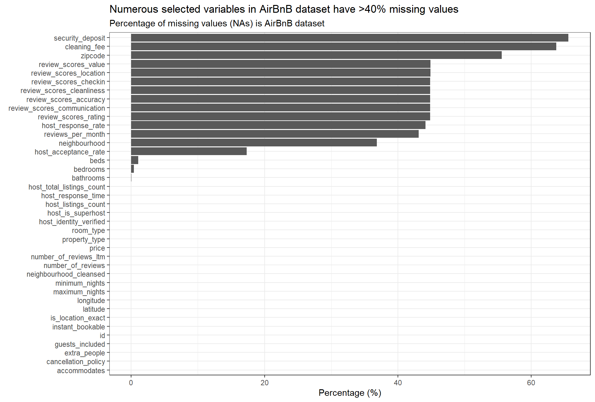
Based on the bar plot we identify additional variables that have a high share (%) of NA values. This is especially relevant for the variables cleaning_fee and security_deposit; we infer that, most likely, there is a high percentage of missing values because there are no cleaning/security fees associated with the stay (i.e. cleaning/security fees = 0). Hence, we are going to assume 0 values in case there is an NA entry. We note that review related variables will require further exploration as there is a high percentage (>40%) of missing values. neighbourhood will be disregarded going forward as the dataset also includes a neighbourhood_cleansed variable where missing values were added.
In order to narrow down the number of different property types (Top 4) and regroup them, we perform a count of listings for the different property types.
Top 4 property types:
- Apartment: 14,428
- Condominium: 4,761
- House: 4,129
- Loft: 2,960
- Other: 10,005
 beijing_properties <- beijing_selected %>%
  #Count the total for the variable property type
    count(property_type) %>%
  #Create a new variable to quantify the percentage
    mutate(percentage = n/sum(n)*100)%>%
  #Arrange in descending order
    arrange(desc(n))
#Choose only the 4 most common properties from the list
beijing_properties <- slice(beijing_properties, -5:-n())

#Create a new row to specify the total number of the first four variables
total <- data.frame("Summary top 4",26278,72.43)
#Specify the names corresponding to the variables we have just added
names(total) <- c("property_type","n","percentage")
#Append the row to the others. Call the new datafrane beijing_properties.New
beijing_properties.New <- rbind(beijing_properties,total)


beijing_properties.New %>%
  #Create a table with package kable extra package

  #col.names just accounts for the names of the variables
  kbl(col.names = c("Property type","Count","Percentage (%)")) %>%
  #Customize the table by defining the font
  kable_material_dark() %>%
  kable_styling(fixed_thead = T, full_width = F, font_size = 14) %>%
row_spec(0, background = "#363640", color = "white")| Property type | Count | Percentage (%) |
|---|---|---|
| Apartment | 14428 | 39.77 |
| Condominium | 4761 | 13.12 |
| House | 4129 | 11.38 |
| Loft | 2960 | 8.16 |
| Summary top 4 | 26278 | 72.43 |
As we can observe, the top 4 property types account for 72.43% of the total. Given that we will only consider Airbnb for travelling purposes, another variable worth exploring is the number of minimum nights.
#Create a variable beijing nights to analyse variable minimum_nights
beijing_nights <- beijing_selected %>%
  #Count the number of minimum nights
  count(minimum_nights)%>%
  #Create a new variable to calculate the percentage
   mutate(percentage = n/sum(n)*100)%>%
  #Arrange in descending order
arrange(desc(n))

# Choose only the 7 most common properties from the list
# beijing_nights <- slice(beijing_nights, -7:-n())

head(beijing_nights, 8) %>%
  #Create a table with package kable extra package
  #col.names just accounts for the names of the variables
  kbl(col.names = c("Minimum nights","Count","Percentage (%)")) %>%
  #Customization
  kable_material_dark() %>%
  kable_styling(fixed_thead = T, full_width = F, font_size = 14) %>%
row_spec(0, background = "#363640", color = "white")| Minimum nights | Count | Percentage (%) |
|---|---|---|
| 1 | 30216 | 83.279 |
| 2 | 2178 | 6.003 |
| 3 | 1024 | 2.822 |
| 30 | 819 | 2.257 |
| 7 | 369 | 1.017 |
| 5 | 368 | 1.014 |
| 15 | 316 | 0.871 |
| 90 | 175 | 0.482 |
We can see that, undoubtedly, the most common value for the number of nights is 1. It accounts for 83.3% of the total values. Having 1 as a minimum seems to indicate that the main purpose is attracting customers since guests can spend as little or as much time as they need to; there are no restrictions. Additionally, it can be observed that there are some minimum night values that are greater than 2 or much greater than 2. This could be due to the hosts seeking to reduce operational costs; if the number of minimum nights is increased, the property won’t have to be cleaned and prepared for the new guests every day.
Subsequently, we proceed to clean the data further by simplifying property type and converting it to a categorical value, and we translate Chinese neighbourhood names into latin names.
beijing_cleaned <- beijing_selected %>%
  # Create a new variable prop_type_simplified
  mutate(prop_type_simplified = case_when(
    #The property type will be assigned to one of the top four if on the list,
    #or to Other if it isn't one of the top four
    property_type %in% c("Apartment","Condominium", "House","Loft") ~ property_type,
    TRUE ~ "Other"),

    # Clean names of neighbourhoods ro be represented in latin letters
    neighbourhood_cleansed = case_when(
           neighbourhood_cleansed == "东城区" ~ "Dongcheng",
           neighbourhood_cleansed == "丰台区 / Fengtai" ~ "Fengtai",
           neighbourhood_cleansed == "大兴区 / Daxing" ~ "Daxing",
           neighbourhood_cleansed == "密云县 / Miyun" ~ "Miyun",
           neighbourhood_cleansed == "平谷区 / Pinggu" ~ "Pinggu",
           neighbourhood_cleansed == "延庆县 / Yanqing" ~ "Yanqing",
           neighbourhood_cleansed == "怀柔区 / Huairou" ~ "Huairou",
           neighbourhood_cleansed == "房山区" ~ "Fangshan",
           neighbourhood_cleansed == "昌平区" ~ "Changping",
           neighbourhood_cleansed == "朝阳区 / Chaoyang" ~ "Chaoyang",
           neighbourhood_cleansed == "海淀区" ~ "Haidian",
           neighbourhood_cleansed == "石景山区" ~ "Shijingshan",
           neighbourhood_cleansed == "西城区" ~ "Xicheng",
           neighbourhood_cleansed == "通州区 / Tongzhou" ~ "Tongzhou",
           neighbourhood_cleansed == "门头沟区 / Mentougou" ~ "Mentougou",
           neighbourhood_cleansed == "顺义区 / Shunyi" ~ "Shunyi")
    ) %>%
  #In the case we have NAs, give them the name N/A
  na_if("N/A")

#Assign 0s to the NA values for cleaning fee and security deposit cases
beijing_cleaned$cleaning_fee[is.na(beijing_cleaned$cleaning_fee)] <- 0
beijing_cleaned$security_deposit[is.na(beijing_cleaned$security_deposit)] <- 0
A further question that we want to address is: how are AirBnB prices distributed in the different neighbourhoods in Beijing?
# Create a dataframe that shows the median prices per night by neighbourhood in Beijing
median_price_dist <- beijing_cleaned %>%
  # select relevant variables
  select(neighbourhood_cleansed, price) %>%
  # group by neighbourhood
  group_by(neighbourhood_cleansed) %>%
  # calculate median price per night
  summarize(median = median(price)) %>%
  #Arrange in decreasing order
  arrange(-median)

# Output bar plot to display price/ night by neighbourhood
ggplot(data = median_price_dist, aes(x = reorder(neighbourhood_cleansed, median), y = median)) +
  geom_bar(stat="identity") +
  labs(title = "AirBnB prices/ night significantly differ by neighbourhood", subtitle = "Median price per night in Beijing by district", x = element_blank(), y = "Median price per night (in Yuan)") +
  #Flip the coordinates
  coord_flip() +
  #Add the theme
  theme_bw()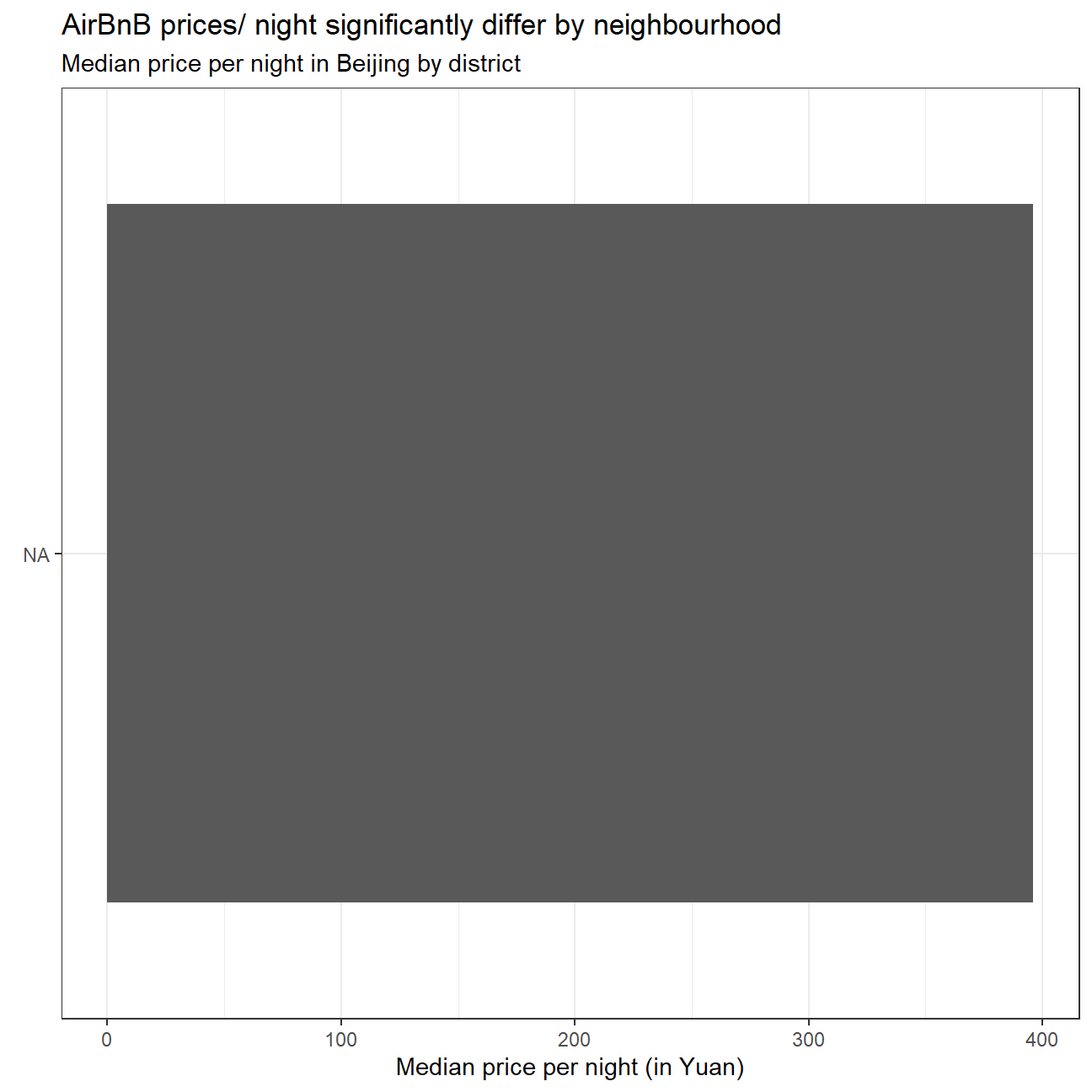
As can be observed in the chart, the median price per night in Beijing for an AirBnB rental differs significantly by neighbourhood.
We use the gathered insights to inform our decision on which districts to regroup in the next step in order to narrow the number of currently 16 different neighbourhoods in the dataset. Therefore, we’ll not only look at geographical location (e.g. directional or distance from city center), but also take into account whether median prices for the district are comparable.
In the following we’ll analyse outliers for the variable of interest price in order to ensure the overall quality of further analyses and to build a accurate regression model. Therefore we’ll remove extreme outliers for price, defined as prices above ¥10,000. Reasons for those outliers in the dataset may be fake listings, hosts that increase prices significantly as they don’t want to rent out the apartment at this particular point, or extremely luxurious apartments.
# refactor variables and filter for relevant AirBnBs

beijing_cleanbase <- beijing_cleaned %>%
  # We filter the dataset for listings where the minimum stay is lower or equal to 4 nights and where at least two people can be accommodated
  filter(minimum_nights <= 4,
         accommodates >= 2,
         price != 0) %>%
  # We perform multiple mutate operations in order to transform the variables into factor variables and relevel them
  mutate(host_response_time = fct_relevel(host_response_time,
                                            "within an hour",
                                            "within a few hours",
                                            "within a day",
                                            "a few days or more"),
         cancellation_policy = fct_relevel(cancellation_policy,
                                           "flexible",
                                           "moderate",
                                           "strict_14_with_grace_period"),
         prop_type_simplified = fct_relevel(prop_type_simplified,
                                          "Apartment",
                                          "Condominium",
                                          "House",
                                          "Loft",
                                          "Other"),
         room_type = fct_relevel(room_type,
                                 "Shared room",
                                 "Private room",
                                 "Entire home/apt"),
         # We regroup the 16 neighbourhoods included in the neighbourhood_cleansed variable based on geographic location in Beijing, factoring in the median price per night for the particular district
         neighbourhood_simplified = case_when(
           # no clear grouping possible for the following neighbourhoods, therefore name stays the same
           neighbourhood_cleansed == "Shunyi" ~ "Shunyi",
           neighbourhood_cleansed == "Chaoyang" ~ "Chaoyang",
           neighbourhood_cleansed == "Huairou" ~ "Huairou",
           # North east Beijing excl. Huairou due to significantly higher price point (Yanqing, Pinggu, Miyun)
           neighbourhood_cleansed == "Yanqing" ~ "Northeast Beijing",
           neighbourhood_cleansed == "Pinggu" ~ "Northeast Beijing",
           neighbourhood_cleansed == "Miyun" ~ "Northeast Beijing",
           # Beijing central (Dongcheng, Xicheng)
           neighbourhood_cleansed == "Dongcheng" ~ "Central Beijing",
           neighbourhood_cleansed == "Xicheng" ~ "Central Beijing",
           # Western Beijing (Shijingshan, Haidian, Fengtai)
           neighbourhood_cleansed == "Shijingshan" ~ "Western Beijing",
           neighbourhood_cleansed == "Haidian" ~ "Western Beijing",
           neighbourhood_cleansed == "Fengtai" ~ "Western Beijing",
           # Belt of Outskirts (Fangshan, Daxing, Tongzhou, Mentougou, Changping)
           neighbourhood_cleansed == "Mentougou" ~ "Beijing Outskirts",
           neighbourhood_cleansed == "Fangshan" ~ "Beijing Outskirts",
           neighbourhood_cleansed == "Changping" ~ "Beijing Outskirts",
           neighbourhood_cleansed == "Daxing" ~ "Beijing Outskirts",
           neighbourhood_cleansed == "Tongzhou" ~ "Beijing Outskirts"
           ),
         # set neighbourhood as factor
         neighbourhood_simplified = as.factor(neighbourhood_simplified),
         # Calculate the price for 4 nights for 2 people
         price_4_nights = case_when(guests_included >= 2 ~ (price*4+cleaning_fee),
                                    TRUE ~ ((price+extra_people)*4+cleaning_fee)),
         price_4_nights_log = log(price_4_nights),
         price_log = (log(price))
         ) %>%
  select(-neighbourhood, -property_type) %>%
  filter(!is.na(host_is_superhost) | !is.na(host_identity_verified)) %>%
  # We add an additional filter to remove all extreme outliers from the price, which we determined by adding 5x the interquartile range to the 3rd quartile
  filter(price < 10000)

# skim(beijing_cleanbase)
Data exploration
Now that we performed an extensive data cleaning process, I will perform some data visualization, showing the most interesting relationsships apparent in the AirBnB dataset.
Let’s show the differences in price/ night by neighbourhood…
# use violin plot to showcase density distribution of price by neighbourhood
beijing_cleanbase %>%
  group_by(neighbourhood_simplified) %>%
  ggplot(aes(x = reorder(factor(neighbourhood_simplified), -price), y = price), colour = neighbourhood_simplified)+
  geom_violin(aes(fill= neighbourhood_simplified))+
  # rescale the y-axis to make the violin plot clearer
  ylim(0,2500)+
  # combine a box plot with the violin plot to show the shape of the distribution, its central value, and its variability
  geom_boxplot(width=0.04, fill = "#FCF9F9",
  # remove the outlier of the boxplot
               outlier.shape = NA)+
  # add median point on the plot and make it in red
  stat_summary(fun.y=median, geom="point", size=1.9, color="black")+
  # add titles and subtitles for the plot as well as rename the axis names.
  labs(title = "Huairou widest distribution of prices in Beijing",
       subtitle = "Density and distribution of prices for each neighbourhood",
       x = "Neighbourhood",
       y = "Price (in ¥)")+
  # reorder the plot to make them in a descending order based on the median price
  scale_x_discrete(limits = c("Huairou", "Northeast Beijing", "Central Beijing",
                              "Chaoyang", "Western Beijing", "Shunyi", "Beijing Outskirts"))+
  scale_fill_manual(values=c("#5E6CC9","#2D866B","#5BC88A","#848A46","#6EA938","#40A3BF","#94D5E2"))+
  theme_bw()+
  # remove the legend
  theme(legend.position = 'none') +
  coord_flip()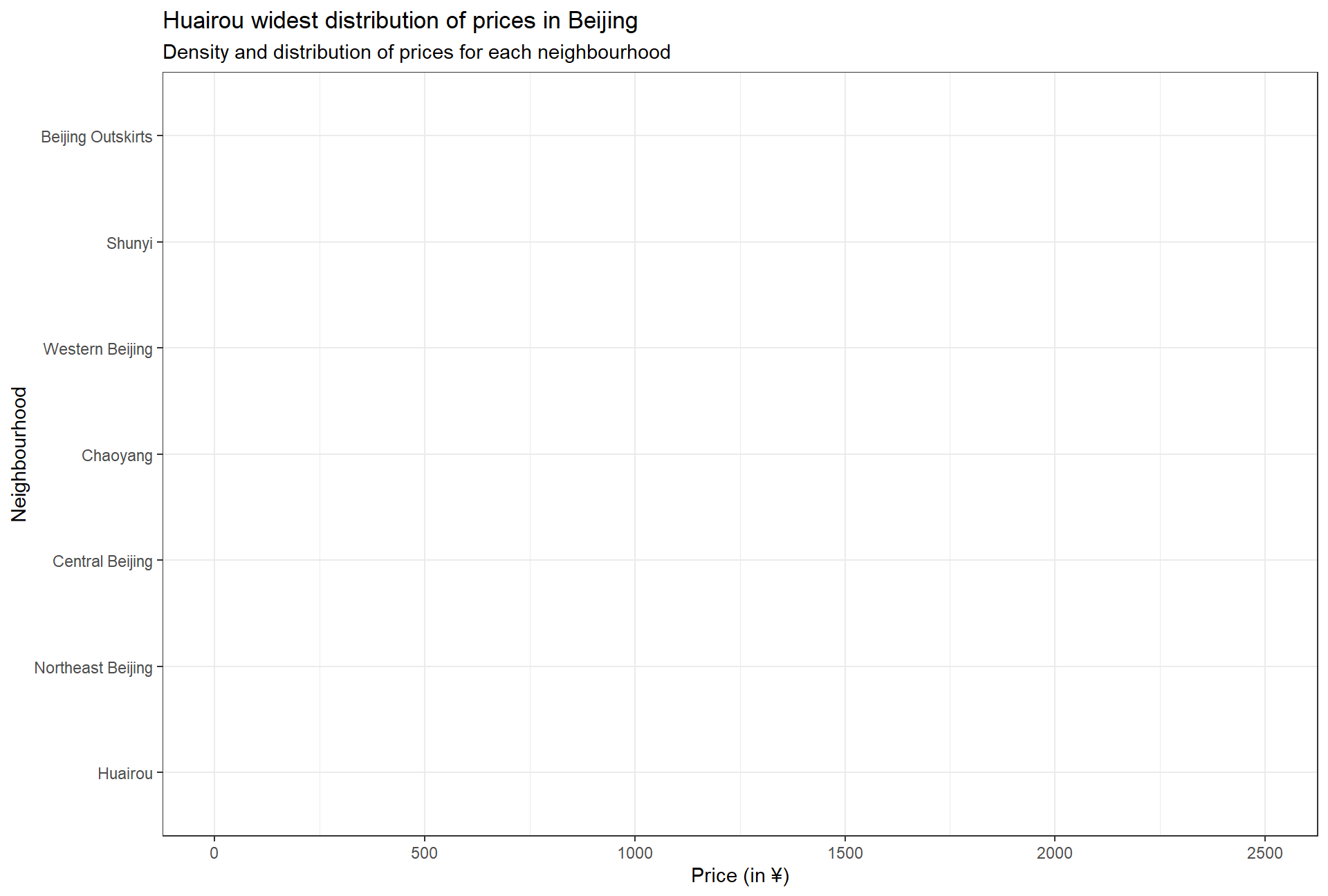
Looking at the distribution of prices it is worth noting that Huairou is the neighbourhood with the widest distribution of prices with the highest median prices/ night at ~¥750. Given the fact that Huairou is located ~50 km outside of central Beijing, the prices are mainly driven by tourists. With the Great Wall of China running through the district and the popular Hong Luo Temple located in Hong Luo mountain, AirBnBs are generally in high demand.
Let’s run some correlation analysis…*
In order to identify potential variables for the regression model, we’ll 1st run a correlation analysis that will be complemented by a ggpairs plot which combines a density plot, histogram and scatter plot with a correlation analysis. We are going to explore the correlations between relevant variables we deem important to our analysis.
# Create a dataframe only including the relevant numeric variables for the correlation
beijing_corr <- beijing_cleanbase %>%
  select(price,
         price_4_nights,
         price_4_nights_log,
         host_response_rate,
         host_acceptance_rate,
         host_listings_count,
         accommodates,
         bedrooms,
         beds,
         bathrooms,
         security_deposit,
         cleaning_fee,
         guests_included,
         extra_people,
         number_of_reviews,
         number_of_reviews_ltm,
         reviews_per_month,
         review_scores_rating,
         review_scores_checkin,
         review_scores_cleanliness,
         review_scores_accuracy,
         review_scores_communication,
         review_scores_location,
         review_scores_value
         )
#create a correlation matrix and then pivot it to together (melt)
cormat <- round(cor(beijing_corr %>% select(-price_4_nights_log), use = "pairwise.complete.obs"),2)
melted_cormat <- melt(cormat)
ggplot(data = melted_cormat, aes(x=Var1, y=Var2, fill=value)) +
geom_tile() +
labs(title = "Correlation Heatmap", x = "", y = "", fill = "Corr. Coeff.") +
scale_fill_gradient(low = "white", high = "green") +
theme(axis.text.x = element_text(angle = 90),
axis.text = element_text(size=8)) 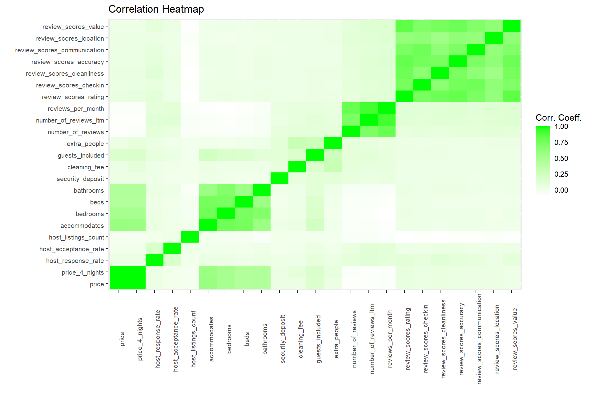 Using this HeatMap we can see 3 highly correlated sets of variables. Those are 1. Ratings metric 2. Reviews/time metrics and 3. Info related to the size of the airBnB. We can see that the ratings metrics (1) have almost no correlation with the price of the unit. From the chart below we can see the correlation facts and determine that review_scores have no correlation with price and will remove them from our consideration. We are going to disregard all columns that have a correlation coeff with price of < |0.05|.
Below we can see that the correlation between each set of variables is very significant but they are not correlated in any way with price.
Using this HeatMap we can see 3 highly correlated sets of variables. Those are 1. Ratings metric 2. Reviews/time metrics and 3. Info related to the size of the airBnB. We can see that the ratings metrics (1) have almost no correlation with the price of the unit. From the chart below we can see the correlation facts and determine that review_scores have no correlation with price and will remove them from our consideration. We are going to disregard all columns that have a correlation coeff with price of < |0.05|.
Below we can see that the correlation between each set of variables is very significant but they are not correlated in any way with price.
#Correlation matrix for ratings related columns
rating_cormat <- beijing_corr %>%
  select(price, review_scores_rating:review_scores_value) %>%
  cor(use = "pairwise.complete.obs") %>%
  round(2)
rating_cormat[upper.tri(rating_cormat)] <- ""
rating_cormat %>%
  kbl() %>%
  kable_material_dark() %>%
  kable_styling(fixed_thead = T, font_size = 12, full_width = F) %>%
row_spec(0, background = "#363640", color = "white")| price | review_scores_rating | review_scores_checkin | review_scores_cleanliness | review_scores_accuracy | review_scores_communication | review_scores_location | review_scores_value | |
|---|---|---|---|---|---|---|---|---|
| price | 1 | |||||||
| review_scores_rating | 0.06 | 1 | ||||||
| review_scores_checkin | 0.05 | 0.75 | 1 | |||||
| review_scores_cleanliness | 0.06 | 0.79 | 0.65 | 1 | ||||
| review_scores_accuracy | 0.05 | 0.82 | 0.76 | 0.74 | 1 | |||
| review_scores_communication | 0.04 | 0.73 | 0.78 | 0.63 | 0.73 | 1 | ||
| review_scores_location | 0.04 | 0.61 | 0.63 | 0.55 | 0.63 | 0.61 | 1 | |
| review_scores_value | 0.02 | 0.84 | 0.71 | 0.75 | 0.79 | 0.7 | 0.63 | 1 |
#Correlation matrix for num reviews related columns
review_cormat <- beijing_corr %>%
  select(price, number_of_reviews:reviews_per_month) %>%
  cor(use = "pairwise.complete.obs") %>%
  round(2)
review_cormat[upper.tri(review_cormat)] <- ""
review_cormat %>%
  kbl() %>%
  kable_material_dark() %>%
  kable_styling(fixed_thead = T, font_size = 12, full_width = F) %>%
row_spec(0, background = "#363640", color = "white") | price | number_of_reviews | number_of_reviews_ltm | reviews_per_month | |
|---|---|---|---|---|
| price | 1 | |||
| number_of_reviews | -0.09 | 1 | ||
| number_of_reviews_ltm | -0.09 | 0.73 | 1 | |
| reviews_per_month | -0.08 | 0.81 | 0.92 | 1 |
We can see that the set of variables related to number of guests has some correlation with price according to our heatmap so we plot it to gain a better understanding. Additionally we expect that the factor of being a superhost (is_superhost) further positively influences the correlation of those variables with price. Therefore we include it in the following plot to analyze the relationship.
beijing_cleanbase %>%
  select(host_is_superhost, price, bedrooms, beds, accommodates, bathrooms, review_scores_rating) %>%
  # Plot the
  GGally::ggpairs(aes(color = host_is_superhost, alpha = 0.4)) +
    labs(title = "Multiple variables related to apartment size and amenities highly correlated with price", subtitle = "")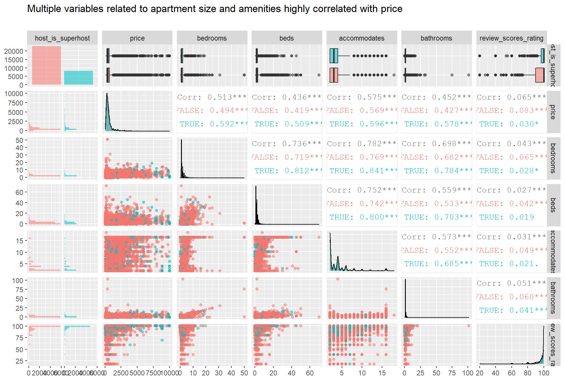
By looking at the scatterplots, we can observe that the relationships between the variables are not linear. If we focus on the price plots, for instance, we can see that there is a wide range of prices concentrated at a low number of bathrooms, bedrooms and beds; most of the price points are located where number of beds, bedrooms and bathrooms is less than 10. There isn’t a clear trend for those points; they are scattered over a wide range of values. In the case of accommodates, the values are spread across the two axes (the price range and the number of accommodates range). Again, there isn’t a linear relationship between the variables, which take multiple and widely spread price values. In the plots seen above, we tested the impact of host_is_superhost on the correlation. We can observe that the correlations are conditional on the value of this categorical variable, as the correlation numbers are not the same when the host_is_superhost takes different values.
Credits
This project was conducted as part of the Applied Analytics
Last updated: 20 September, 2020